
Heard about antenna tuning but couldn’t get past the mathematics behind it? Here is a quick and practical guide on how to go along with antenna tuning for your own IoT device.
What is antenna tuning?
An antenna has a resistance, capacitance and inductance. These are determined by antenna’s physical properties which include the shape, size, material and also by the environment. When a high frequency signal is fed to an antenna to radiate, not all the power is radiated by the antenna but a small portion of it is reflected back to the source. These reflected waves creates ‘Standing Waves’ in the transmission line and results in losses. Minimum reflection is obtained when source impedance is equal to the load impedance. To reduce these reflections and ultimately power loss, the load impedance(i.e. The antenna) should be equal to the source impedance(usually 50 ohm or otherwise described). Antenna tuning is basically, the process of matching the antenna impedance with source impedance. If the antenna already has an impedance equal to the source impedance, there is no need of tuning.
Why tune an antenna?
Antenna is probably the most important part of a wireless system, as it is responsible for sending and receiving the data on the physical layer. A properly tuned antenna can help in many ways. It can increase the working range and can also help in reducing the power consumption of wireless device.
VSWR, S11, Return Loss:
These are the most commonly used and heard terms when doing antenna tuning. VSWR stands for Voltage Standing Wave Ratio. It is a function of the reflection coefficient, which describes the power reflected back from the antenna. The reflection coefficient is known as s11 or return loss. The VSWR is always a real and positive number for antennas. The smaller the VSWR is, the better the antenna is matched to the transmission line and the more power is delivered to the antenna. The minimum VSWR is 1.0. In this case, no power is reflected from the antenna, which is ideal. In general, if the VSWR is under 2 the antenna match is considered very good and little would be gained by impedance matching.
| VSWR | (s11) | Reflected Power (%) | Reflected Power (dB) |
| 1.0 | 0.000 | 0.00 | -Infinity |
| 1.5 | 0.200 | 4.0 | -14.0 |
| 2.0 | 0.333 | 11.1 | -9.55 |
| 2.5 | 0.429 | 18.4 | -7.36 |
| 3.0 | 0.500 | 25.0 | -6.00 |
| 3.5 | 0.556 | 30.9 | -5.10 |
| 4.0 | 0.600 | 36.0 | -4.44 |
As can be seen from the table, VSWR of 2 corresponds to 11.1% of reflected power. This means that to the antenna, 89.9% of power is transmitted. VSWR of 1.5 will increase this transmitted power to 96%, which isn’t very big jump. Therefore, reducing the VSWR from 2 to 1.8-1.7 won’t bring in much improvements to your antenna tuning.
Antenna choice
Commonly used antenna types:
Whip Antenna:
Whip antennas are simple in construction and are readily available in market. They are Omnidirectional except for along the length of the antenna (Donut Shaped Radiation Pattern). These are usually very efficient and are available with simple Plug and use standard connector (SMA, U.FL). Their major disadvantage is Size and therefore these are not suitable to put inside a box.
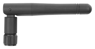 Whip Antenna
Dipole Antenna:
Dipole antennas are simple in construction and don’t require any additional ground plane. Their radiation pattern is similar to Whip Antennas, Omnidirectional except for along the length of the dipole (Donut Shaped). Various modifications exist of dipole antennas, Half-wave, Monopole, Folded Dipole, Short Dipole and so on. Their major disadvantage is also their size.
PCB antenna:
PCB Antennas are small and compact. They do not require any matching components as the matching is done by changing the length of the antenna. They are mainly used where there is space constraint, for example, inside Mobile Phones. Their major disadvantage is that these are not as efficient as Dipole antenna. Another thing to keep in mind is that the antenna may have to be tuned again, if any changes are made on the PCB. For example, the antenna tuning may go off, if the laminate, or PCB thickness, PCB material or some other components is changed.
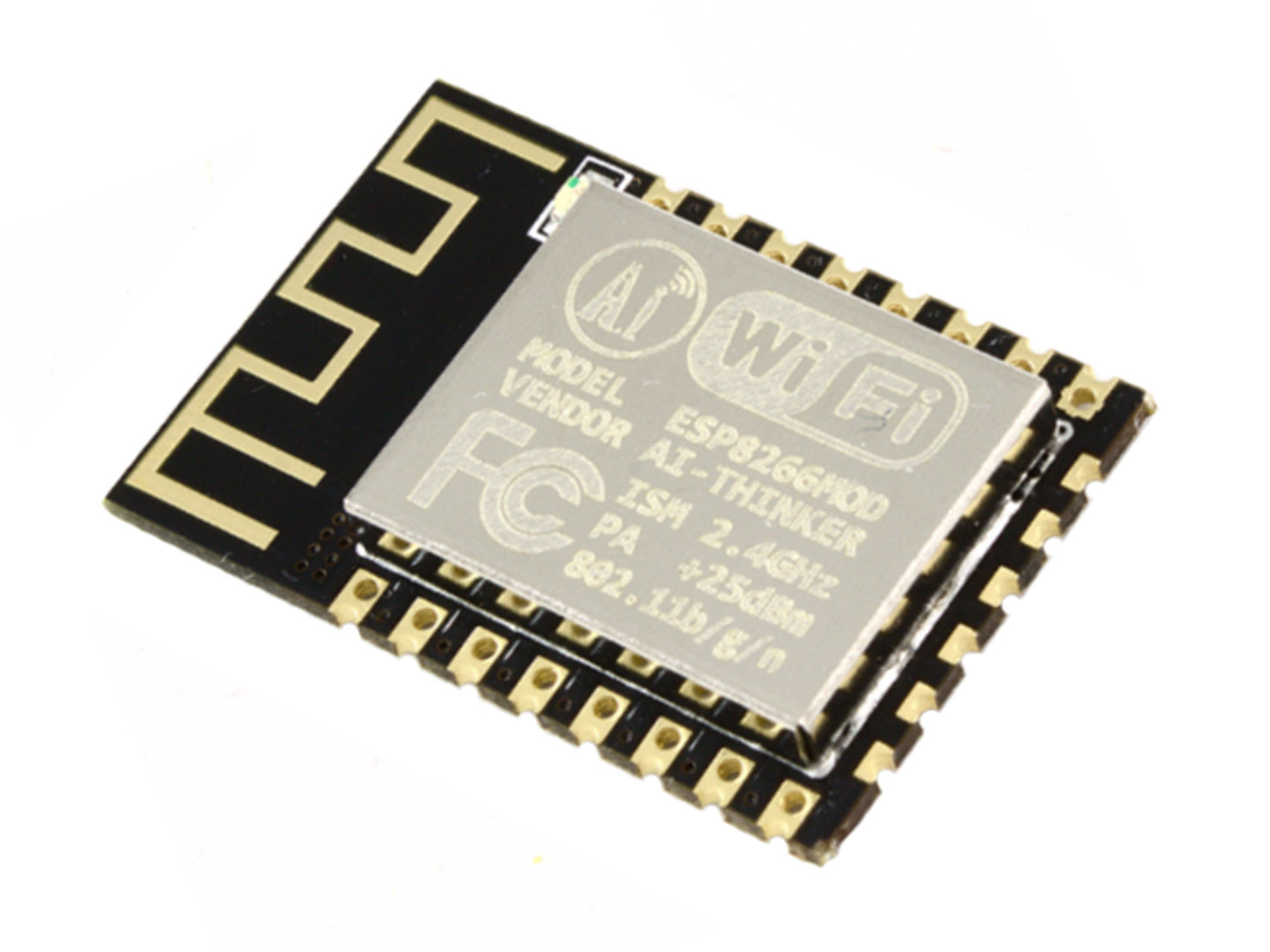
ESP-12F WiFi Module with PCB Antenna
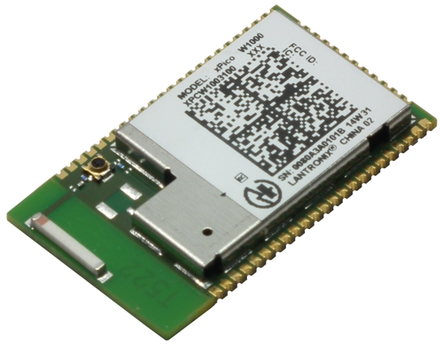
Dielectric resonator antenna (Chip Antenna):
These are very small and compact. They also are almost Omnidirectional in nature. They typically require a ground plane. Their Input Impedance varies and thus matching is required in almost all cases. Their major disadvantage is that they are not as efficient as Dipole Antennas. In almost all the cases these need proper tuning with a matching circuit and matching components introduce additional loss.
Working Frequency range
The size of antenna decides the working frequency range. Larger the size of antenna, smaller is the resonant frequency and vice versa. The antenna chosen should be according to the working frequency range required.
Bandwidth
The bandwidth of an antenna refers to the range of frequencies over which the antenna can operate correctly. The antenna’s bandwidth is the number of Hz for which the antenna will exhibit an VSWR less than 2:1 (or return loss is less than -10dB).
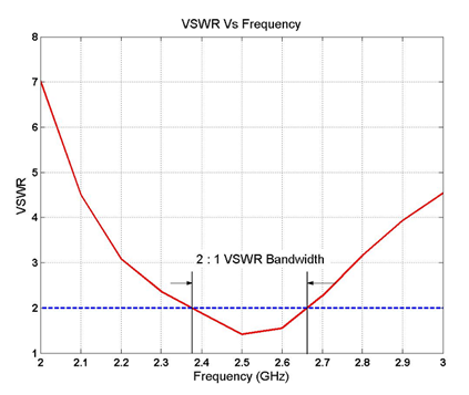
Bandwidth is from 2.4GHz to 2.7GHz
When the antenna is inside a box or a case, the antenna parameters may change compared to the antenna in Free Space. To compensate for these shifts, wide-band antenna is preferred.
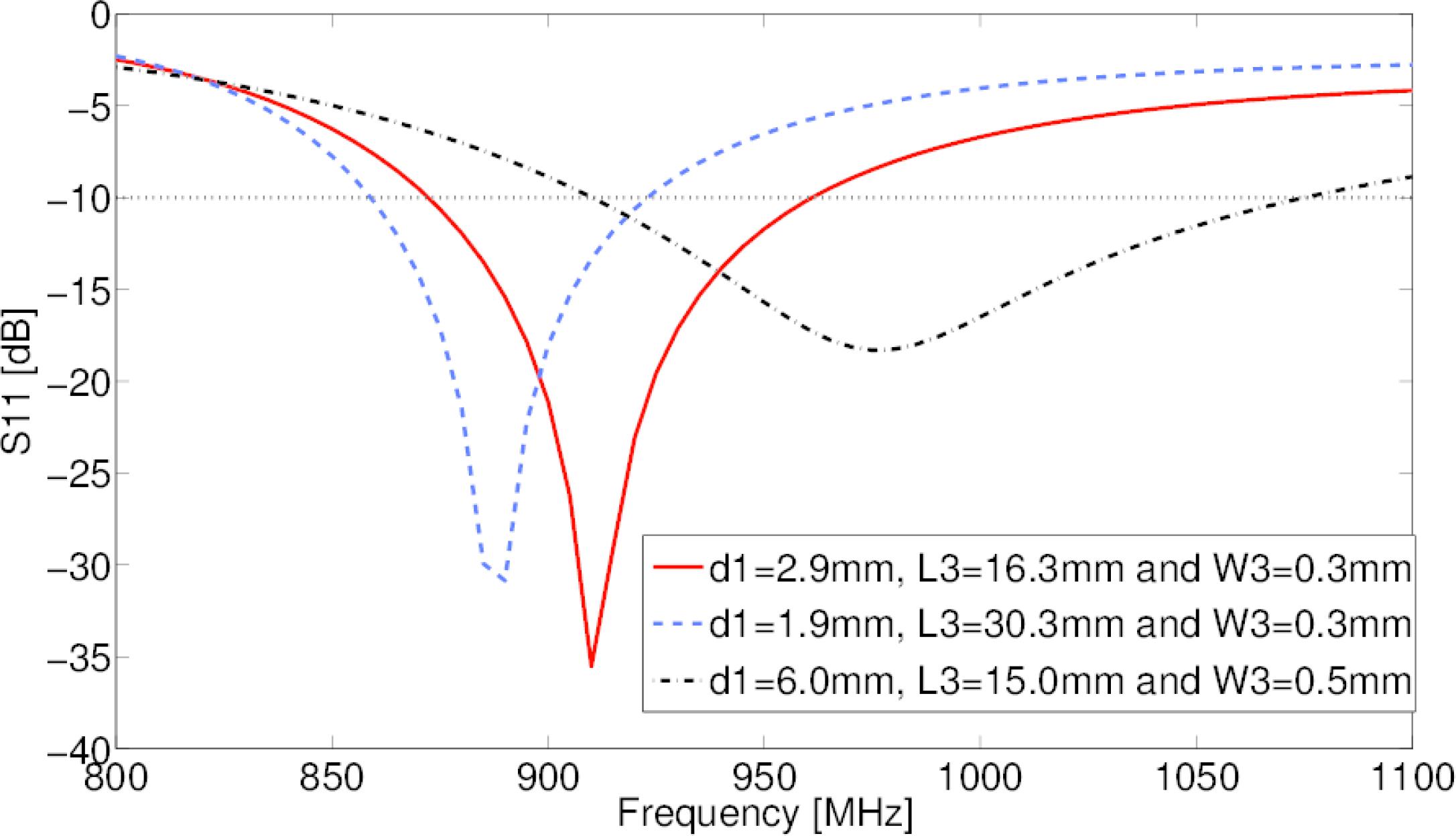
The graph below compares the bandwidth of three antennas with different physical parameters. The black dotted line exhibits the highest bandwidth while the red dotted line has the lowest bandwidth. Note that, the return loss is also increased with an increase in bandwidth. The bandwidth and the return loss have to be compromised.
Size and Space constraint
When putting an antenna inside a box, sometimes there might be space constraint. Generally, Losses will be more in a smaller sized antenna as compared to a proper sized one. It is always advised to choose a proper sized antenna if space is not a constraint or if the antenna can be put outside the box (Whip Antenna).
Gain, Radiation Pattern and Directivity
An antenna with high directivity will provide better range and performance but in one specific direction only. An isotropic antenna (Omnidirectional) will have to compromise on range.
Gain of an antenna can be a positive or negative value. A positive value tells how much more the antenna will radiate as compared to an isotropic antenna and a negative value tells how less the antenna will radiate in comparison to isotropic antenna.
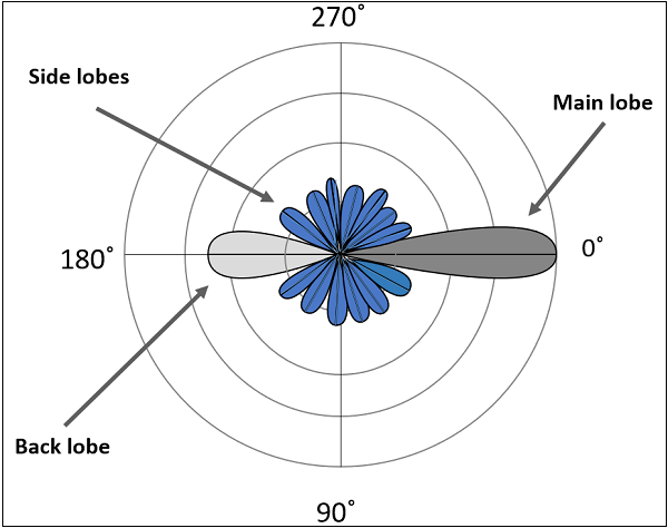
Radiation pattern is the plot describing in which directions the antenna will radiate. It has main and side lobes. Antenna will radiate the most in the direction of the main lobe, while it may not radiate in some specific directions (In between lobes).
For example in this radiation pattern, the major portion of radiation will be along the Main and back lobe, but there will be very small radiation along the Side lobes.
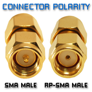
Connector Type
How the antenna will be connected to the PCB will depend upon the Connector Type. Most antenna choices are available with SMA and U.FL connectors. The Connector also depends on space available on PCB.
 SMA Connector
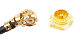
U.FL Connector
Tools Required
Hardware
VNA (Vector Network Analyzer) :
There are lots of different VNA’s available in the market but they are usually very costly. The VNA that we used is called ‘miniVNA’ and is fairly economical compared to others. It is a USB based VNA, with no display and thus has to be connected to a computer to view the results.
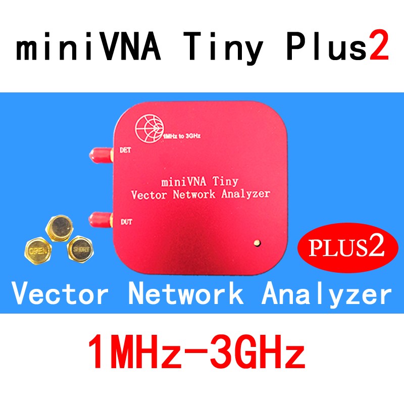
Here is a link to buy it from aliexpress: miniVNA Aliexpress
Calibration Kit:
A calibration kit is used to calibrate a VNA and has 3 connectors, short, open and 50 ohm impedance. It has to bought externally if not supplied with the VNA. The MiniVNA has these included inside the box.
Matching components:
For tuning the antenna, matching components (inductors and capacitors) of various different values will be required . While buying these components, make sure that their ESR rating is less. Lower the ESR, lower is the stray inductive and capacitive effects.
Here is a Bill Of Materials (BOM) of different valued components that we bought from lcsc.com : BOM
This can be uploaded directly at their website for quick buy.
Connector converters:
Sometimes there is a need of converting one connector type to another. For example a SMA to U.FL or SMA male to SMA female. For this purpose, different converters are available which can convert from one connector type to another.
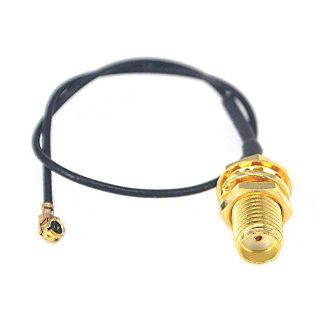 SMA to U.FL Connector
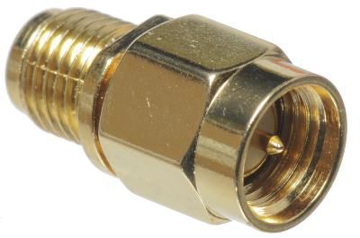 SMA male to female Connector
Software
Software for VNA and calibration
The software for VNA will depend upon the VNA being used. Please refer to the specific VNA’s website for more information.
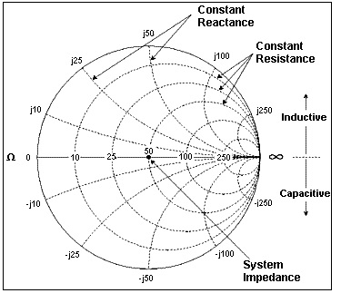
Smith Chart plot:
Smith Chart is a tool to visualise the complex impedance of an antenna as a function of frequency. These are extremely helpful for impedance matching. It is used to display an actual (physical) antenna’s impedance when measured on a Vector Network Analyzer (VNA). The value of matching components can be calculated very easily using a Smith Chart.
 Smith Chart
A software is available for plotting Smith Chart and calculating components values: https://www.w0qe.com/SimSmith.html
PCB Guidelines
Antenna placement
While placing an antenna on a PCB, guidelines given in the antenna datasheet should be followed as much as possible. Make sure there are no metal parts near the antenna as that may cause the antenna parameters to change. The feedline connecting the antenna to the source should be equal to the source impedance as the feedline forms a part of the transmission line connecting the antenna. For tuning purposes, a Pi network should be added just before the antenna placement (if antenna needs to be tuned) preferably in ‘0403’ packaging.
How to tune antenna:
This section will give a practical idea on how to go along with the antenna tuning. With each step there is a Use Case, which describes how we did it to tune our antenna.
VNA Calibration
The very first step of antenna tuning is VNA calibration. VNA Calibration or Vector error correction is the process of characterising the systematic errors of the network analyser system by measuring known devices called calibration standards. Subsequently, the effects of the characterised systematic errors are mathematically removed from raw measurements. Calibration should be done as close as possible to the point of interest. Long cables in between the VNA and the DUT (Device Under Test) can add phase delays which will give wrong measurements.
How to do VNA calibration on PCB
To check an antenna which is not mounted on to the PCB, the VNA calibration can be done directly with the help of the calibration kit. Refer to your specific VNA documentation on how to calibrate the VNA. However, to check an antenna mounted on PCB, the calibration has to be done with the PCB itself. This is because the feedline will actually form a part of the transmission line feeding the antenna. Therefore, it also needs to be taken into account. For the calibration, take a good quality small length coaxial cable and solder the cable on the PCB as shown in the image. The cable should be soldered just before the point where feedline starts.
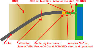
The OPEN calibration can be done just by keeping the PI circuit open. The SHORT calibration can be done by shorting the feedline with ground and the LOAD calibration can be done by connecting a resistor in between the feedline and the ground (The PI circuit can be used to put the resistor). Choose a resistor which has correct impedance, and has tolerance of 1% or better. After the calibration is done, save the calibration (please refer to VNA documentation) for future use.
Use Case
Keeping the above points in mind, we prepared our own PCB for calibration.
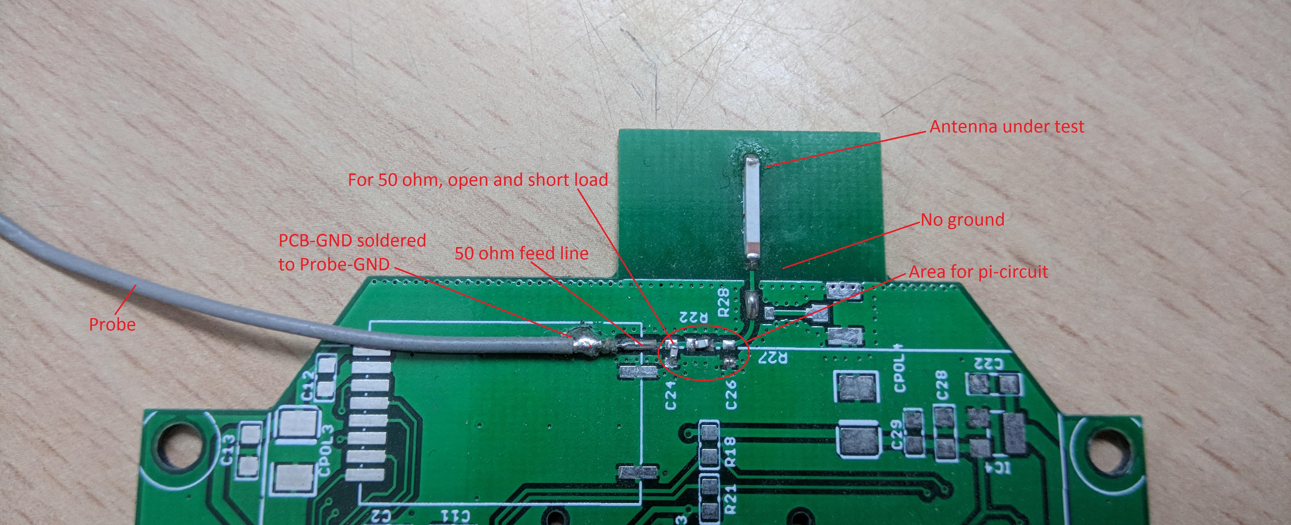
For OPEN calibration, we removed C24, C26, R22, R28 and R27. For SHORT calibration, we put a 0 (zero) ohm resistor at C24 and kept everything else the same and for LOAD calibration, a 50 ohm resistor was installed at C24 keeping everything else the same. This generated the calibration which we used for antenna measurement.
Initial Antenna measurement
Once the calibration is done, you can start with the antenna measurement. Connect the VNA with the antenna, without any matching components. If the antenna needs to be inside a box, put it inside the box and mount it like it has to be in final version. Check the Return Loss and VSWR in the frequency range of interest. Anything below -10 dB return loss/VSWR < 2:1 is good enough. There will be no major benefit of going from -10 dB to -20 dB.
This is because at VSWR 2:1, only 11.1% of total power transmitted to the antenna is reflected back. That means 89.9% of total power is transmitted by the antenna. At VSWR 1.5:1, 4% of total power is reflected and 96% power is transmitted by antenna. There will be no significant difference in 89.9% and 96% transmitted power.
If the antenna response in the desired frequency range is already below -10dB, the antenna is tuned. If not, then proceed further on how to tune.
Use Case
We tested our antenna without any matching component, with the calibration generated above. These were the results.
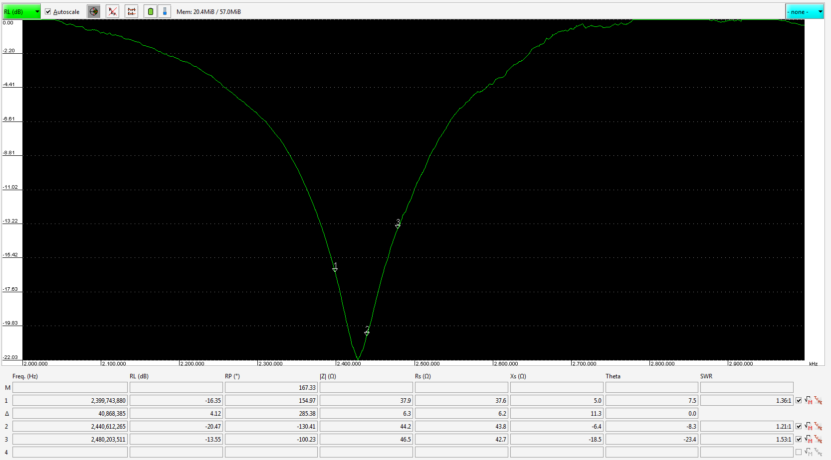
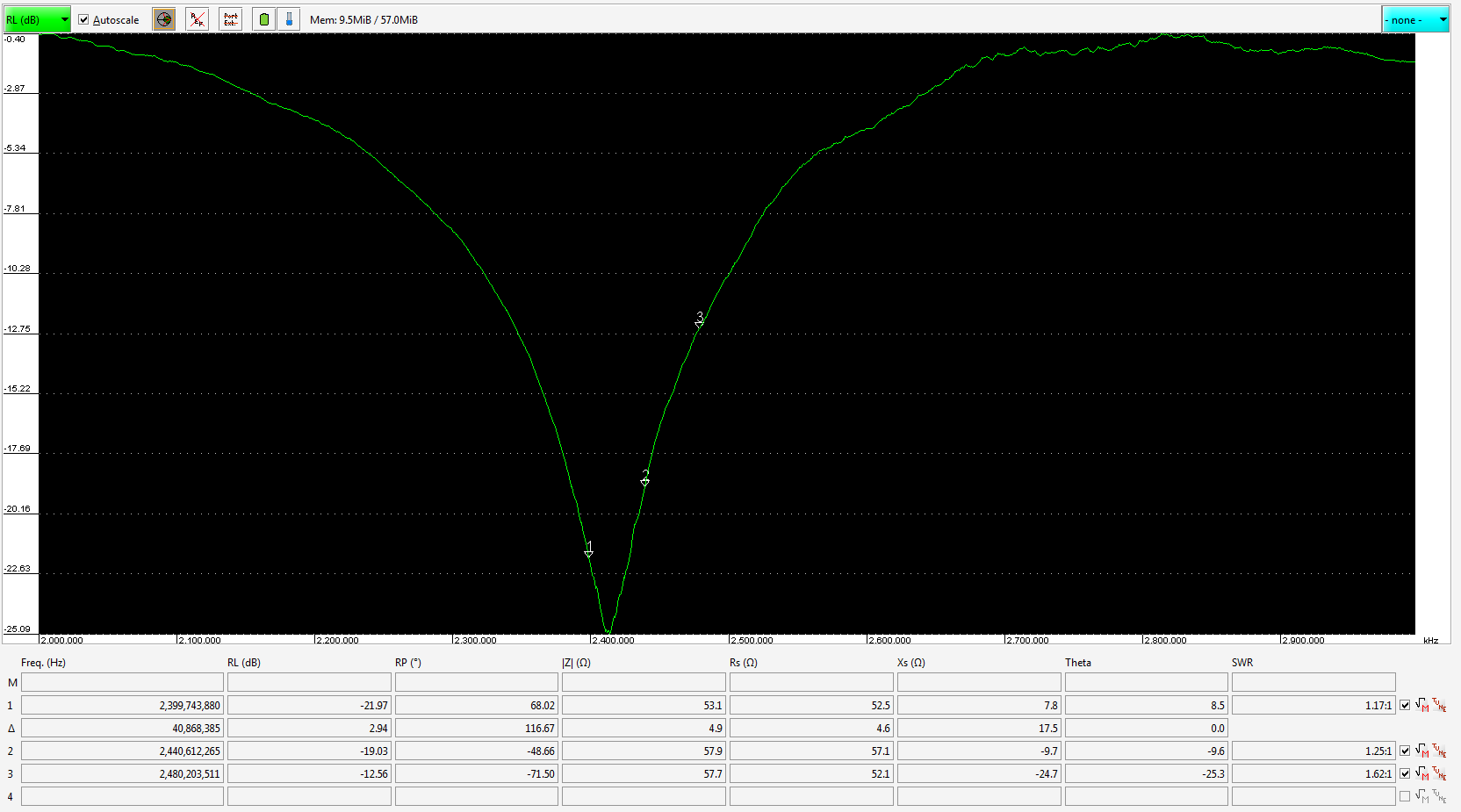
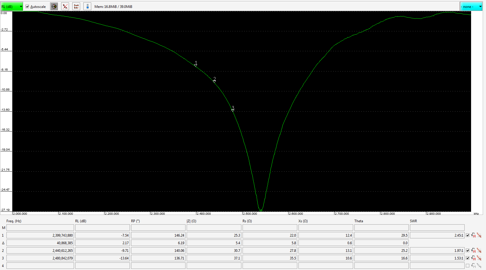 Return Loss Plot vs Frequency
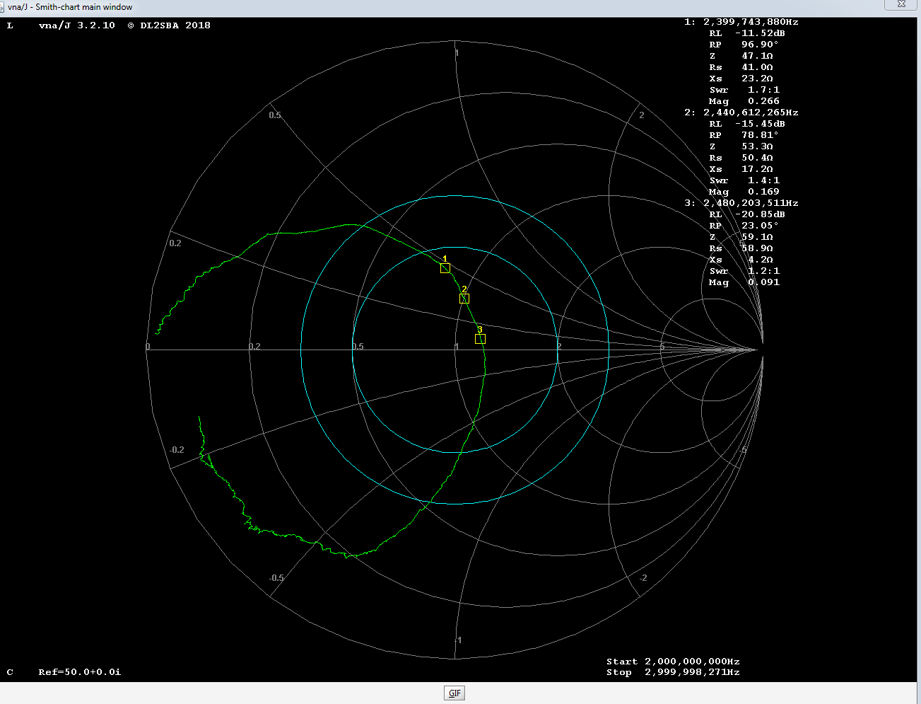
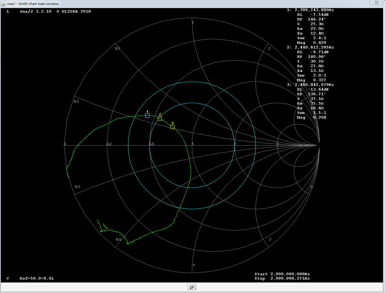 Smith Chart
As can be seen the return loss ‘dip’ is somewhere around 2.5 GHz but the required frequency range was 2.4 GHz ISM band.
Decide which point to tune
Depending upon the use case, the antenna may have to work on a single frequency or a wide range of frequency. If the antenna has to work on a single frequency, then the point of interest is that single point alone. For example- An antenna may be required to work at 868.5 MHz only. In this case a single point is of interest. In some cases, the antenna has to work over a range of frequencies. For example- an antenna working in 2.4 GHz ISM band has to work from 2400 MHz to 2483.5 MHz. If an antenna has to work in a range of frequencies, usually the centre point of the frequency range is the point of interest. It may shift in either direction depending upon the application use case. If higher frequency range has to be preferred, the point of interest can shift towards the higher range and same if a lower frequency range is desired. Once the point of interest is decided, check it on the Smith Chart plotted by the VNA. The goal is to somehow bring it to the centre area of Smith Chart which represents perfect match. To shift the point of interest towards the centre of Smith Chart, matching components are used.
Use Case:
In our application, the point of interest was set to 2440 MHz, as the required frequency range was 2.4 GHz ISM band. The goal was set to bring point ‘2’ (2440 MHz) in the above graphs as close as possible to the centre of the Smith Chart.
Calculate matching components value
To find out the matching components and to calculate their values, a little knowledge about how points shift on a Smith Chart is required. A very basic and practical approach is shown here, to know more on Smith Chart, please check the article here:
http://www.antenna-theory.com/tutorial/smith/chart.php
Using the Smith Chart calculator, decide on which matching components to use and calculate their values. The goal is to get the required tuning point as close as possible to the centre point of Smith Chart. Sometimes it may not be possible to move the point to the centre location with one component only. In that case, multiple components have to be used.
Smith Chart Tutorial:
The smith chart is a tool to visualise the complex impedance of an antenna as a function of frequency. The points plotted on the Smith Chart are thus complex in nature, i.e. they have a real value and a complex value. The real value is plotted on the X-axis and the complex value is plotted on the Y-axis. A point plotted on the Smith Chart can move along some specific path only. These paths are called the ‘Constant Resistance Circles’ and ‘Constant Conductance Circles’. A Smith Chart with both the ‘Constant Resistance Circles’ and ‘Constant Conductance Circles’ is called ‘Immittance Smith Chart’.
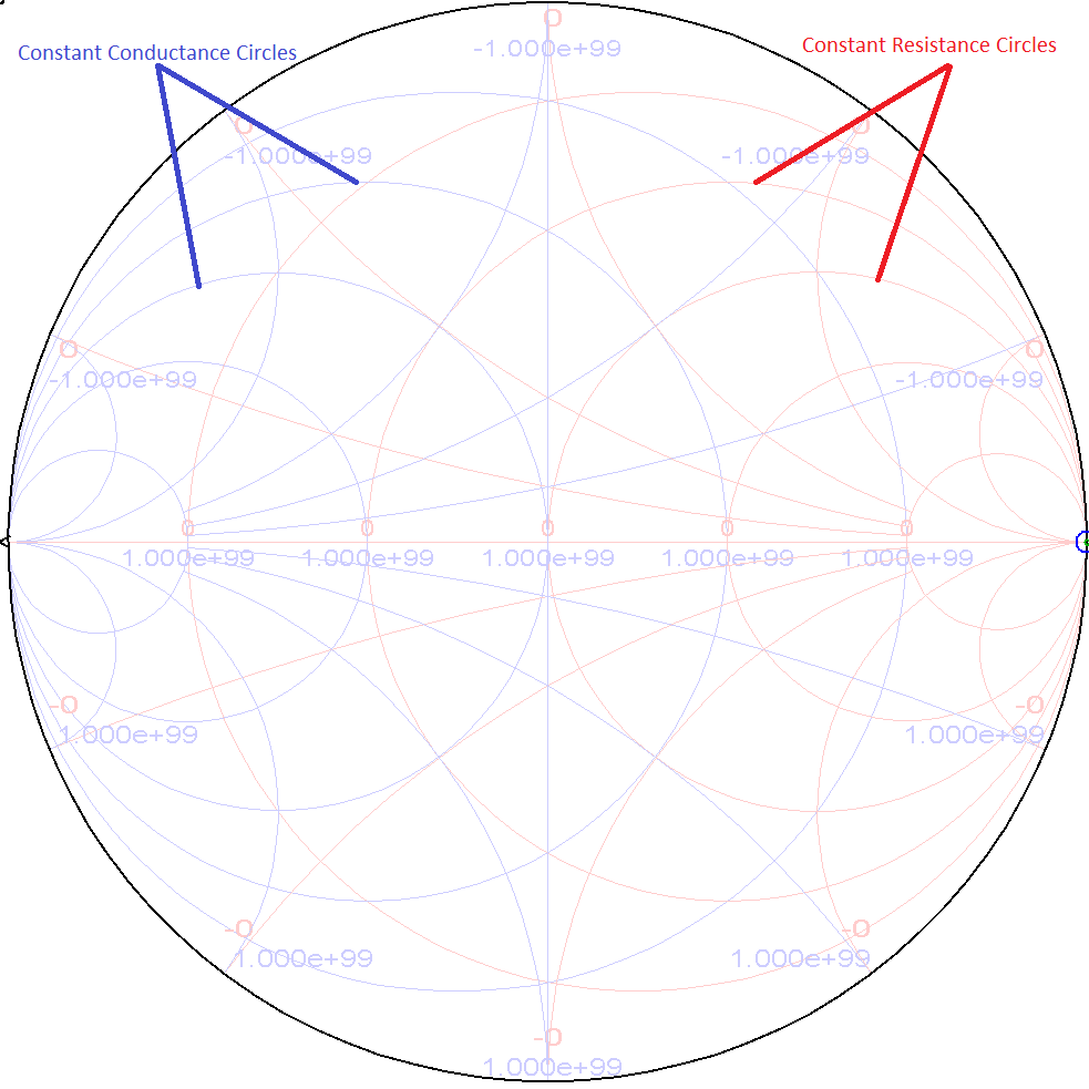
Immitance Smith Chart
How Points Move on Smith Chart
To move a point along the specific paths, a matching component is required (inductor or capacitor).
In all below cases, Red point indicates the starting point and Blue indicates the end point.
A series inductor will shift the point in clockwise direction along the Constant Resistance Circle.
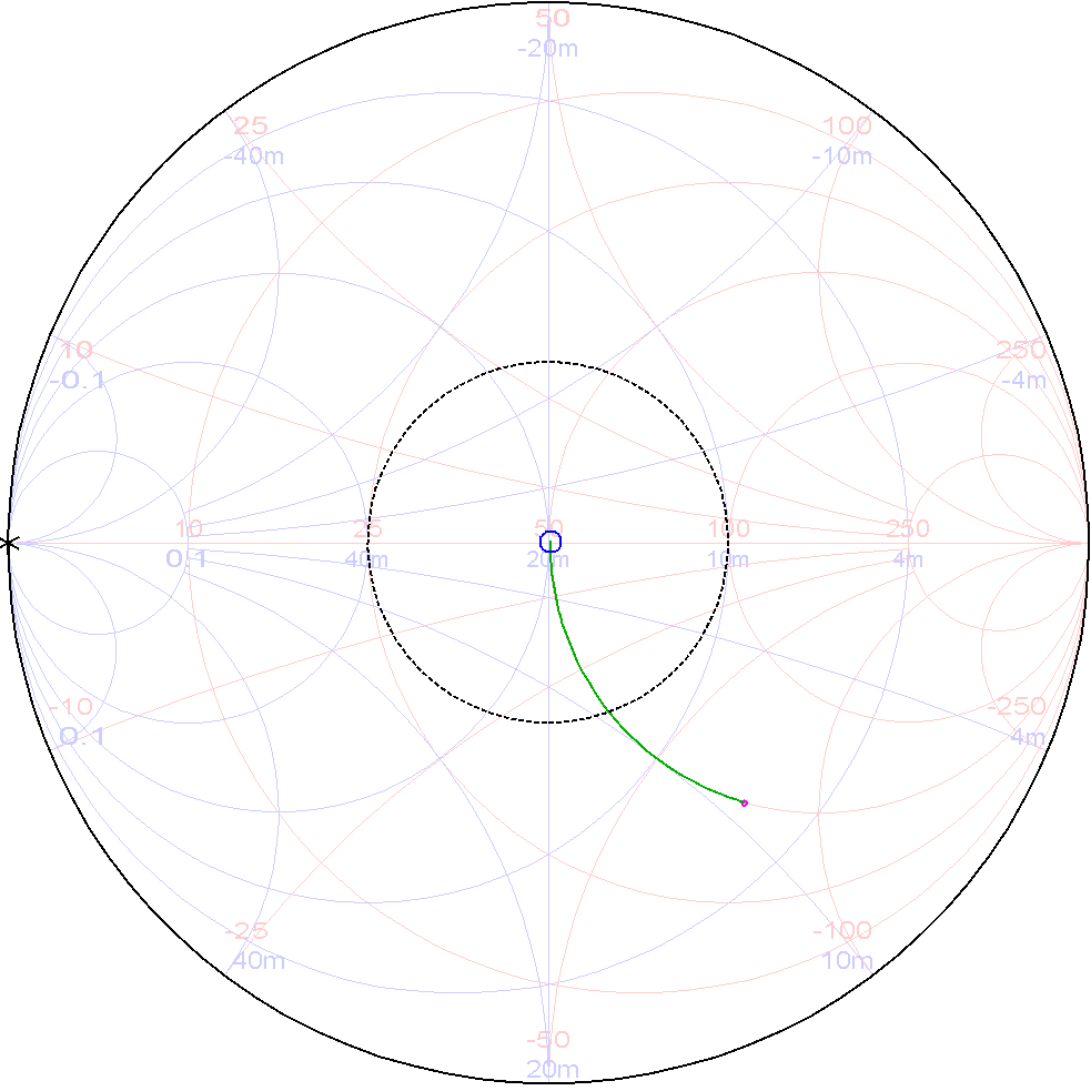
A series capacitor will shift the point in anticlockwise direction along the Constant Resistance Circle.
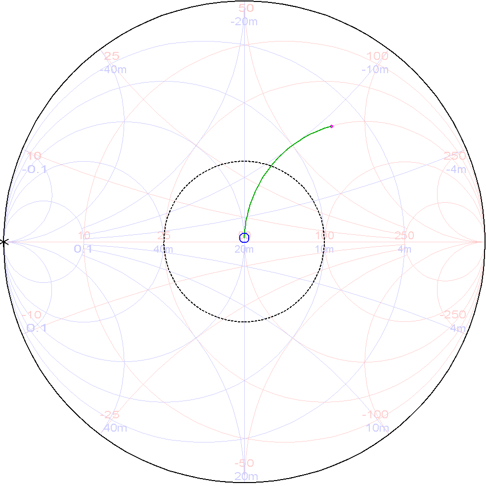
A parallel inductor will move a point in counter clockwise direction along the constant conductance circle.
A parallel capacitor will move a point in clockwise direction along the constant conductance circle.
Use case:
Using the SimSmith tool, matching components values were calculated. We decided to use a L circuit, as only one component was not enough to bring the point ‘2’ (2440 MHz) to the centre.
The matching component values calculated were:
- Parallel Capacitor: 1 pF
- Series Inductor: 1 nH
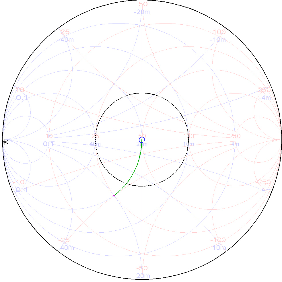
The theoretical calculated point shift was like this.
Testing the antenna behaviour with calculated components values
Using the above calculated components value, do the antenna measurement again. If the frequency of interest seems to be well below -10dB, tuning is done.
Use case:
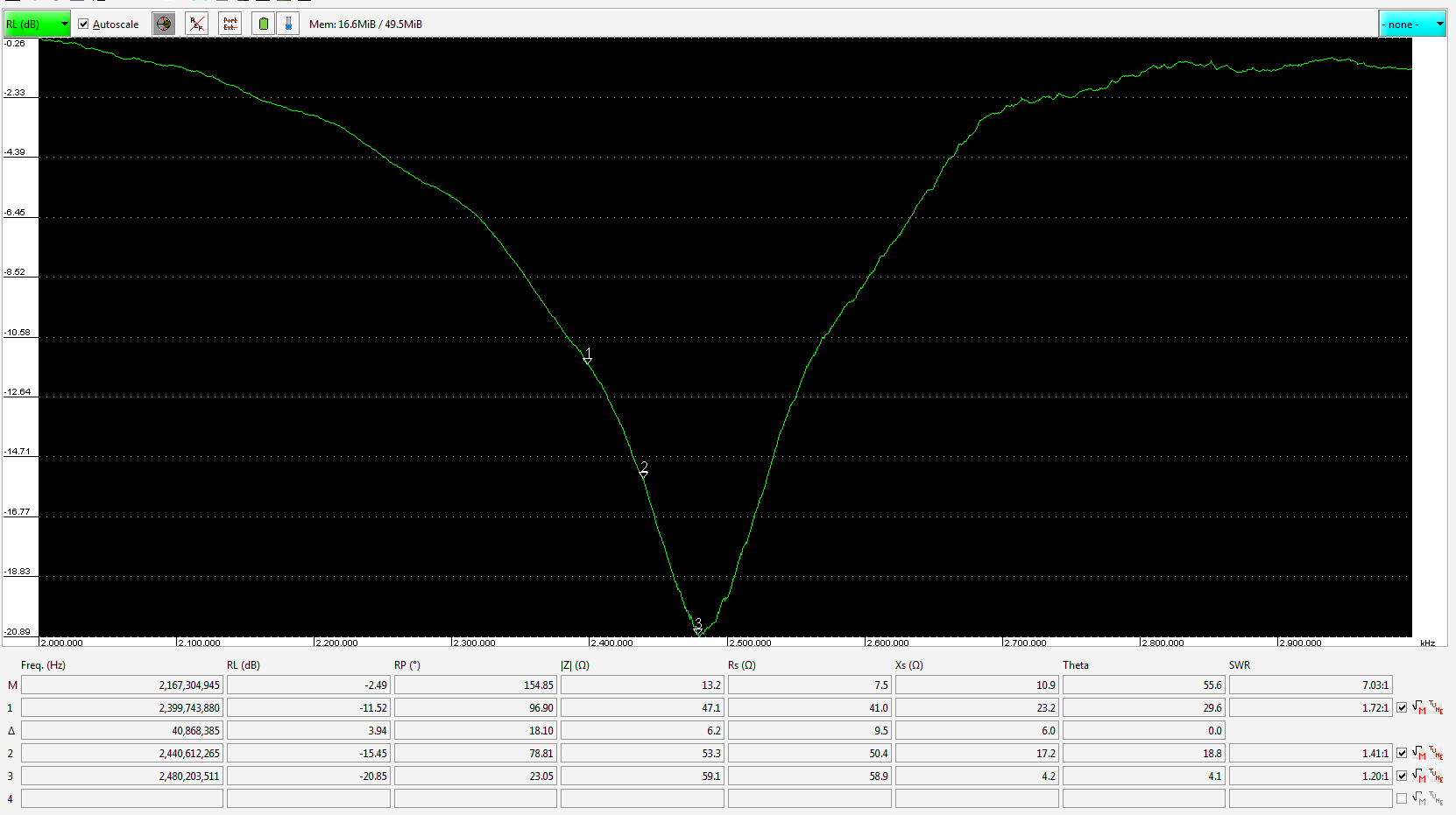
With the above calculated values, the measurements were taken again. The result obtained was pretty close to the theoretical calculation although not exact. The antenna seemed to be tuned very well for 2.4 GHz ISM band, but our requirement was to get the higher frequency range better.
 Return Loss Plot vs Frequency
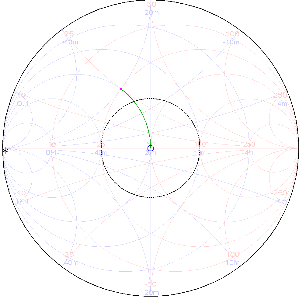
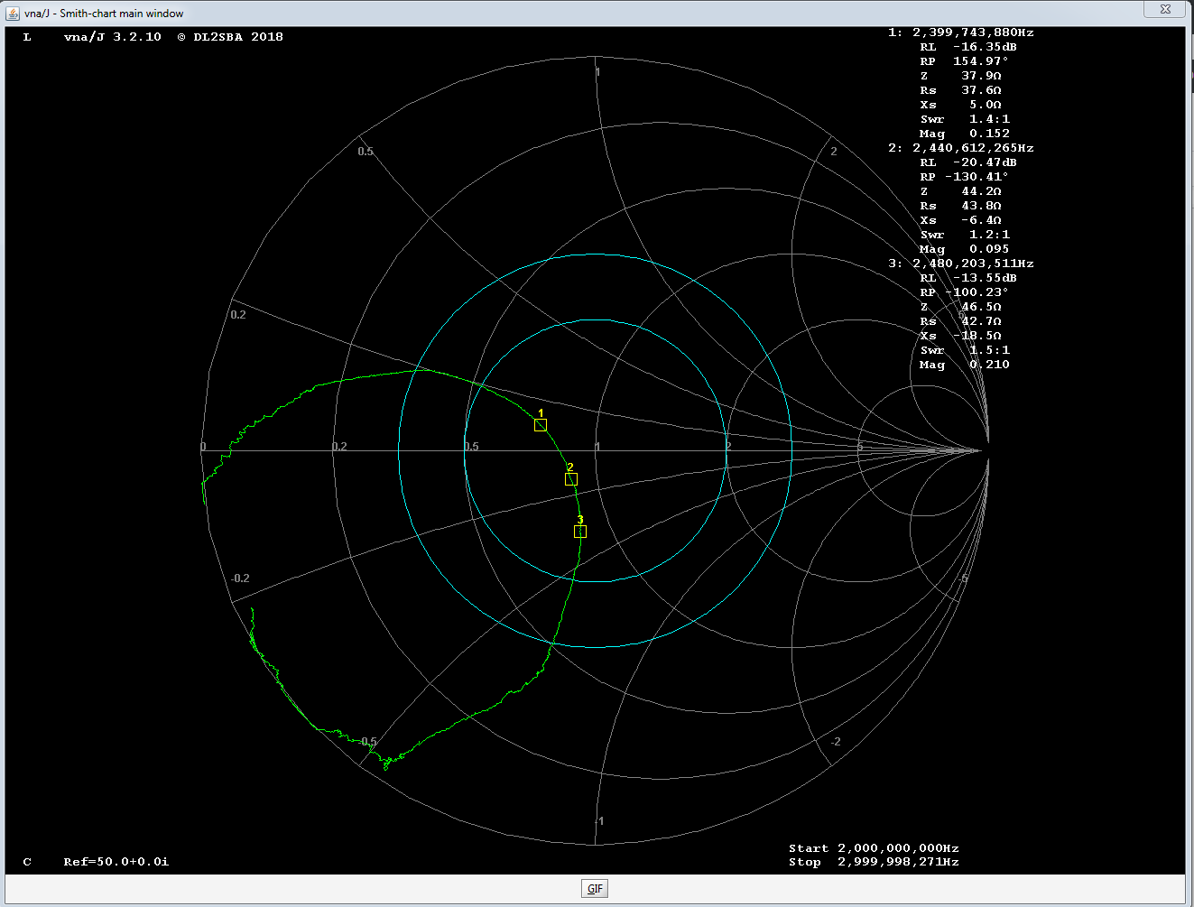 Smith Chart
Repeat above steps till the required point is matched properly
The theoretical calculated matching component value may not provide the exact same response practically as there is always parasitic capacitance in an inductor and parasitic inductance in a capacitor. While doing theoretical calculations, either all these need to be considered or some practical hit and trial is required.
Use case:
Attempt #1:
The initial tuning seemed fine, but our requirement was to get the upper frequency ranges better. The component calculations were done again, this time trying to get the point ‘3’ (2480 MHz) as close as possible to the centre of Smith Chart.
Calculated values:
- Parallel Capacitor: 1 pF
- Series Inductor: 1.5 nH
The results obtained were this
 Return Loss plot vs Frequency
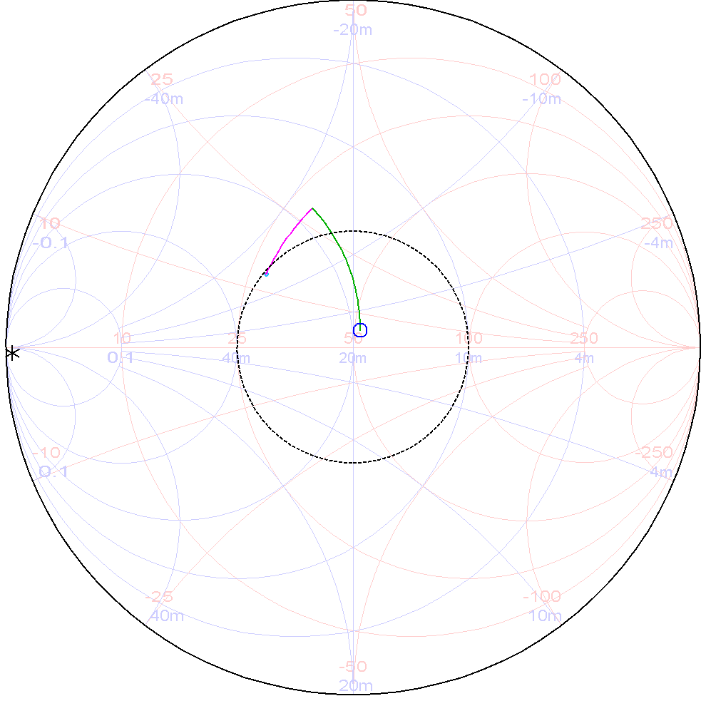
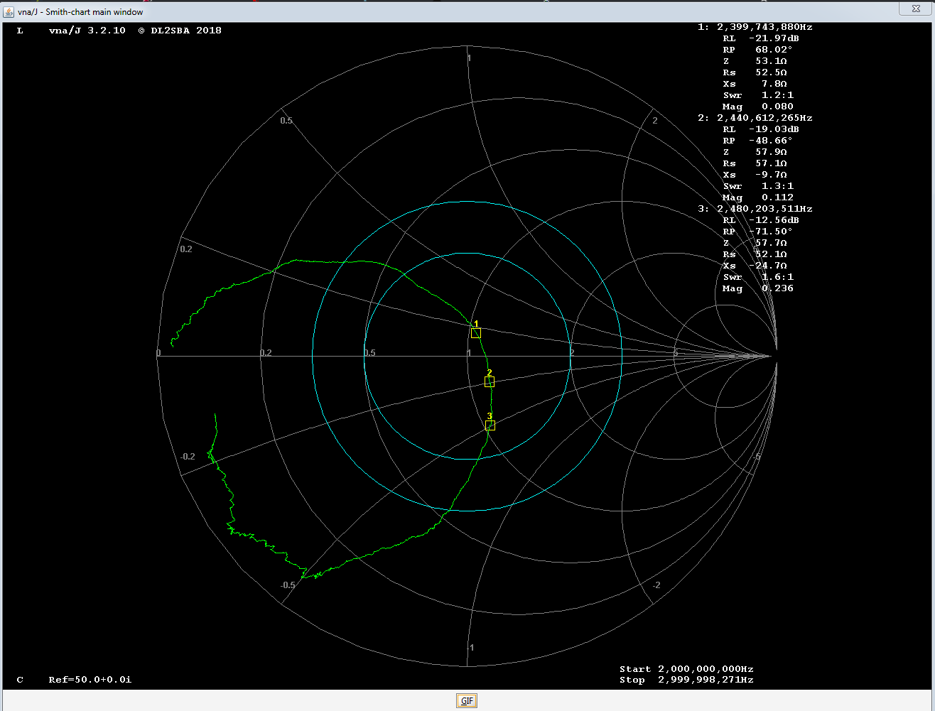 Smith Chart
Attempt #2:
Calculated values:
- Parallel Capacitor: 0.5 pF
- Series Inductor: 1.5 nH
 Smith Chart
Test the device with the tuned antenna
When it seems that the antenna is tuned, test the device in real life scenario.
Use Case:
With the antenna tuned, we decided to test it in real conditions. Before tuning, the antenna worked over a very short range (~10 meters). With the tuning done, the range was increased and so was the transmission speeds. The device is now able to transmit big chunks of data from even 2 floors up with concrete ceilings and walls in between reliably. In open area, we were able to achieve over 90 m (295 feet) of direct line-of-sight range which is pretty good considering an Omnidirectional antenna on a battery powered device working at 2 Mbps on air data rate.
That’s it! A very basic introduction to antenna tuning. We hope you learned something from this article.
Please let us know how we did in the comment section below.