
Facial recognition technology is on the rise and has already made its way into every aspect of our lives. From smartphones, to retail, to offices, to parks… it is everywhere. If you are just getting started with computer vision, then face recognition is a must do project for you. Here in this guide, I seek to present all the existing facial recognition algorithms and how they work. We will explore classical techniques like LBPH, EigenFaces, Fischerfaces as well as Deep Learning techniques such as FaceNet and DeepFace.
Terminology
Before we get started, we need to clarify some terminology as people often get confused if they don’t understand the nuances.
Face recognition is different from face detection:
- Face Detection: the goal is to find bounding box coordinates around the faces in the image so that it may be cropped and used for face recognition.
- Face Recognition: the goal is identify the individual.
There are 2 modes that a face recognition system can operate in:
- Face Verification: It is used for authentication of a person. It compares the input facial image with the facial image of the authenticating user. This is 1v1 matching or One on One matching. Although seemingly simple, this is hard to achieve as there can be no room for false positives!
- Facial Identification or recognition: This involves trying to match a given face against a database of faces. The challenge here is to come up with a similarity metric that can be used to quantify how similar a face is to another face. This is a 1vN comparison.
Techniques
The list of currently practiced techniques for face recognition are:
- Eigenfaces (1991)
- Local Binary Patterns Histograms (LBPH) (1996)
- Fisherfaces (1997)
- Deep Learning (2014)
Each method lays out a different approach for extracting facial features from the image pixels. Some methods such as Eigenfaces and Fisherfaces are similar. Whereas some are completely non-intuitive to our understanding such as Deep Learning. In this guide, we will try to cover the gist of how each technique works along with links to code examples.
Local Binary Patterns Histograms (LBPH).
Being one of the easier face recognition algorithms, it is also one of the oldest techniques
Local Binary Pattern (LBP) is a simple yet very efficient texture operator which labels the pixels of an image by thresholding the neighborhood of each pixel and encodes the result as a binary number.
It was first described in 1994 and has since been found to be a powerful feature for texture classification. As in HOG, we use Histograms to represent and bin the LBP. This allows us to represent the face images with a simple data vector. It has further been determined that when LBP is combined with the histograms of oriented gradients (HOG) descriptor, it improves the detection performance considerably on some datasets. As LBP is a visual descriptor it can also be used for face recognition tasks.
Note: Read more about the LBPH here: http://www.scholarpedia.org/article/Local_Binary_Patterns
Operation
Calculation of Local Binary Patterns is done as follows
- Convert facial image to grayscale.
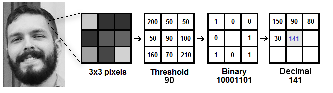
- Select a window of 3×3 pixels. It will be a 3×3 matrix containing the intensity of each pixel (0~255).
- Take the central value of the matrix and use it to threshold the neighboring pixels.
- For each neighbor of the central value (threshold), we set a new binary value. We set 1 for values equal or higher than the threshold and 0 for values lower than the threshold.
- Now, the matrix will contain only binary values (ignoring the central value). We need to concatenate each binary value from each position from the matrix line by line into a new binary value (e.g. 10001101). Note: some authors use other approaches to concatenate the binary values (e.g. clockwise direction), but the final result will be the same.
- Then, we convert this binary value to a decimal value and set it to the central value of the matrix, which is actually a pixel from the original image.
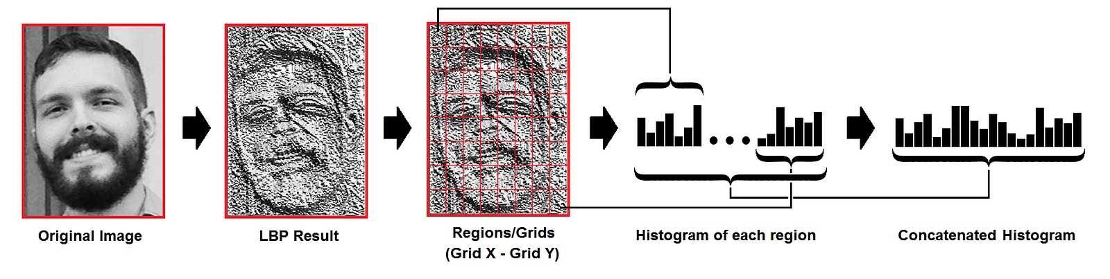
- At the end of this procedure (LBP procedure), we have a new image which represents better the characteristics of the original image.
- Extract histogram of the LBP patterns by dividing the image into a Grid.
- As we have an image in grayscale, each histogram (from each grid) will contain only 256 positions (0~255) representing the occurrences of each pixel intensity.
- Then, we need to concatenate each histogram to create a new and bigger histogram. Supposing we have 8×8 grids, we will have 8x8x256=16.384 positions in the final histogram. The final histogram represents the characteristics of the image original image.
Performing the face recognition
Face images are compared by converting both into LBPH vectors and then calculating the distance between two histograms, for example: euclidean distance, chi-square, absolute value, etc. For ex, Euclidean distance can be calculated based on the following formula:
The distance metric can also be thresholded to ensure the match is accurate enough.
One may also train an SVM or Random Forest classifier on a set of these vectors for quick 1vN classification/prediction. This is the LBPH technique in a nutshell.
Conclusions
- LBPH is one of the easiest face recognition algorithms.
- It can represent local features in the images.
- It is possible to get great results mainly in a controlled environment.
- It is robust against monotonic gray scale transformations.
Eigen Faces
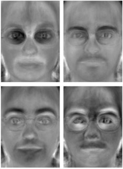
Eigenfaces is the oldest and one of the simplest face recognition methods. It works quite reliably in most controlled environments and with sufficiently large datasets.
In Eigenfaces algorithm, we “project” face images into a low dimensional space in which they can be compared efficiently. The assumption is that intra-face distances (i.e. distances between images of the same person) will be smaller than inter-face distances (the distance between pictures of different people) in the low dimensional space. This projection of the face on to a lower dimension is a form of feature extraction – the dimensions of this space correspond to a feature. Howerver, unlike standard feature extraction with a fixed extractor, for Eigenfaces we learn the feature extractor from the image data. Once we’ve extracted the features, classification can be performed using any standard technique. 1-nearest-neighbour classifiers are the standard choice for the Eigenfaces algorithm.
The lower dimensional space used by the Eigenfaces algorithm is learned through a process called Principle Component Analysis (PCA). PCA is an unsupervised dimensionality reduction technique.
The PCA algorithm finds a set of orthogonal axes (i.e. axes at right angles) that best describe the variance of the data such that the first axis is oriented along the direction of highest variance.
Operation
- First, we gather a set of face images. The faces must be frontal, aligned and cropped to the face region. They must capture sufficient lighting variations for each face.
- Convert to grayscale and normalize by dividing each pixel by 255. Then subtract the mean face (calculated for the dataset).
- Calculate covariance matrix for the training set.
- Learn the feature extractor: Calculate eigenvalues and eigenvectors of the covariance matrix – eigenvectors are the orthonormal basis i.e. these are the principal components that define the face space.
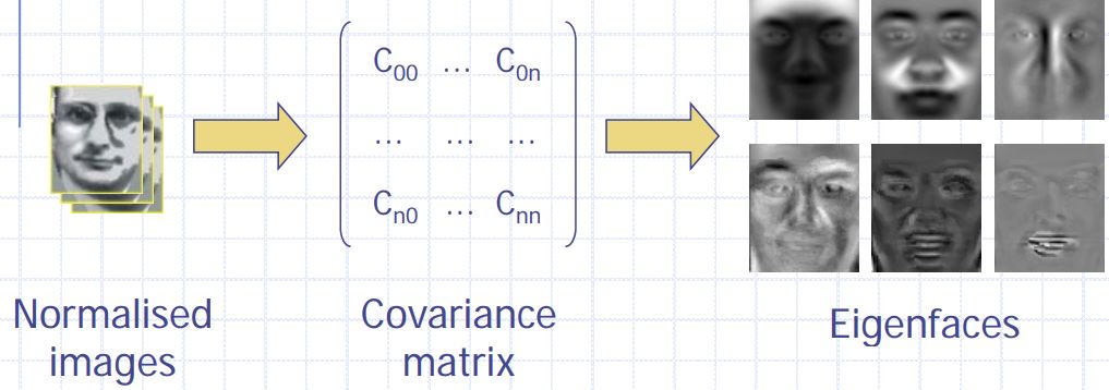
- Essentially, the eigenfaces are dimensions along which a given face’s components should be calculated. The resulting components are the extracted features.
- Use the learned feature extractor to extract features from all face images.
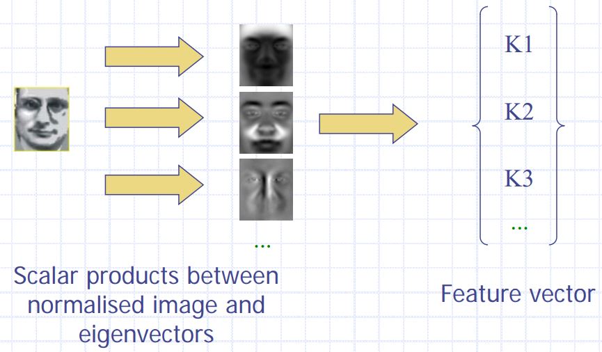
- Use the feature vectors to perform comparison
- One can use euclidean distance calculation or train a linear classifier like SVM, Nearest neighbour etc. to classify the faces.
Conclusions
- Eigenfaces is one of the simplest and oldest face recognition algorithms.
- It is relatively fast compared to other techniques for classifying faces
- The feature extractor must be retrained if large number of new faces are added to the system
- It is not accurate enough by itself and needs boosting methods for improvement.
Fischer Faces
Fisherface is a technique similar to Eigenfaces but it is geared to improve clustering of classes. While Eigenfaces relies on PCA, Fischer faces relies on LDA (aka Fischer’s LDA) for dimensionality reduction.
The FLDA maximizes ratio of between-class scatter to that of within-class scatter. It, therefore, works better than PCA for the purpose of discrimination.
The Fisherface is especially useful when facial images have large variations in illumination and facial expression. Fisherface removes the first three principal components responsible for light intensity changes.
Fisherface is more complex than Eigenface in finding the projection of face space. Calculation of ratio of between-class scatter to within-class scatter requires a lot of processing time. Besides, due to the need of better classification, the dimension of projection in face space is not as compact as Eigenface. This, results in larger storage of the face and more processing time in recognition.

Operation
- First, we gather a set of face images. The faces must be frontal, aligned and cropped to the face region. They must capture sufficient lighting variations for each face.
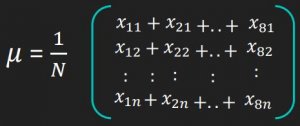
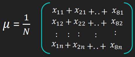
- Compute the average of all faces of all persons in the dataset
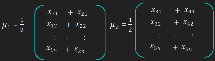
- For each person, compute the average of all images and subtract it from the images to form the training images for that person
- Construct the Imagematrix
Xwith each column representing an image. Each image is a assigned to a class in the corresponding class vectorC. - Project
Xinto the(N-c)-dimensional subspace asPwith the rotation matrixWPcaidentified by a Principal Component Analysis, whereNis the number of samples inXcis unique number of classes (length(unique(C)))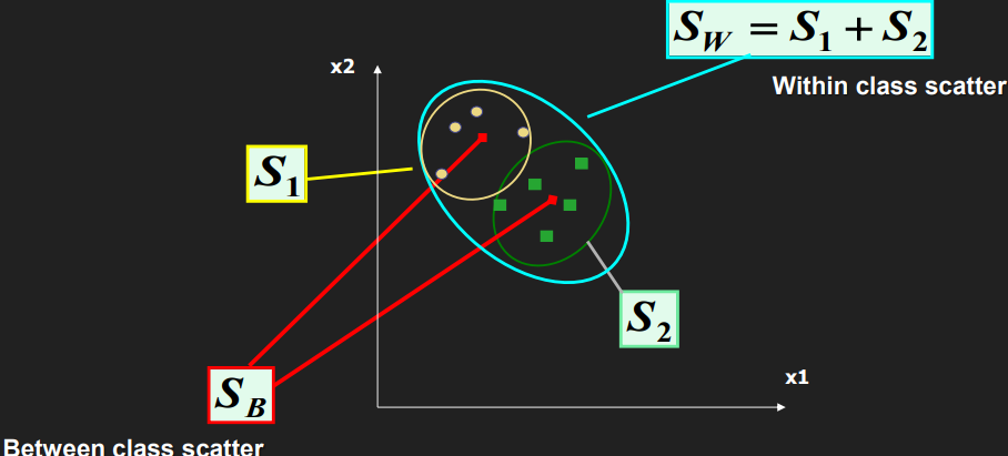
- Calculate the between-classes scatter of the projection
PasSb = \sum_{i=1}^{c} N_i*(mean_i - mean)*(mean_i - mean)^T, wheremeanis the total mean ofPmean_iis the mean of classiinPN_iis the number of samples for classi
- Calculate the within-classes scatter of
PasSw = \sum_{i=1}^{c} \sum_{x_k \in X_i} (x_k - mean_i) * (x_k - mean_i)^T, whereX_iare the samples of classix_kis a sample ofX_imean_iis the mean of classiinP
- Apply a standard Linear Discriminant Analysis and maximize the ratio of the determinant of between-class scatter and within-class scatter. The solution is given by the set of generalized eigenvectors
WfldofSbandSwcorresponding to their eigenvalue. The rank ofSbis atmost(c-1), so there are only(c-1)non-zero eigenvalues, cut off the rest. - Finally obtain the Fisherfaces by
W = WPca * Wfld.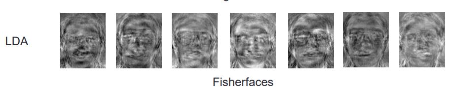
Conclusion
Fischerfaces yields much better recognition performance than eigen faces. However, it loses the ability to reconstruct faces because the Eigenspace is lost. Also, Fischer faces greatly reduces the dimensionality of the images making small template sizes.
In the next, part of the article we will look into Deep Learning techniques for face recognition.
References:
- https://towardsdatascience.com/face-recognition-how-lbph-works-90ec258c3d6b
- http://www.scholarpedia.org/article/Fisherfaces
- https://onionesquereality.wordpress.com/2009/02/11/face-recognition-using-eigenfaces-and-distance-classifiers-a-tutorial/